Flexibility Is Not a Number: Comparing Flexibility Measures in Control, Process Design, Energy Systems, and AI

Control theory, process design, energy systems, and AI all built measures of preserved future capability. They are not the same object, and moving one across the boundary is wrong in ways you can predict.

Every engineer who has sized a battery, chosen a horizon, or argued about how much headroom to leave in a controller has made a flexibility argument. Keep options open. Do not paint yourself into a corner. Preserve the ability to respond to something you cannot yet name.

The intuition is universal, and it has been formalized at least seven different ways. Process systems engineering has a flexibility index. Control theory has viability kernels and terminal sets. Reinforcement learning has empowerment. Power systems have flexibility envelopes. Economics has quasi-option value. AI safety has POWER.

The usual reading of this is convergence: many fields circling the same underlying quantity, waiting for someone to write it down properly. That reading is wrong, and expensively so. These are not seven approximations to one number. They are measures of different properties, under different assumptions, answering different questions — and the differences are precisely where a metric borrowed from one field silently misleads in another.

This article proposes four questions that any flexibility measure must answer, uses them to separate the seven, and argues that the interesting territory is the region none of them occupy.

Seven objects, and why they are not interchangeable

Start with what each community actually computes.

The flexibility index (Swaney & Grossmann 1985) asks how far process parameters can deviate from nominal before no operating point remains feasible. It is the largest scaling of a deviation box that stays inside the feasible region — a scalar, obtained from a three-level max-min-max program.

The viability kernel (Aubin 1991; 2009 reprint) is the set of states from which some admissible trajectory keeps the system inside its constraint set forever. Note the existential quantifier: the nondeterminism in the dynamics is resolved in the agent's favor, which makes it choice rather than adversarial uncertainty — the adversarial versions are the invariance and discriminating kernels. And note the type: this is a set, not a number. It tells you whether a state is survivable. It does not rank two survivable states by how much freedom each retains.

MPC recursive feasibility (Mayne, Rawlings, Rao & Scokaert 2000) delivers X_N, the set of states admitting a feasible N-step plan into an invariant terminal set. Its central property is that X_N is positively invariant under the MPC law, and monotone non-decreasing in N: a longer horizon is literally a larger set of situations you can handle.

Empowerment (Klyubin, Polani & Nehaniv 2005) is the channel capacity from an action sequence to the agent's future sensor reading (the state, in the fully observed case) — the maximum over distributions on action sequences of the mutual information between those actions and what the agent subsequently perceives. It measures how many futures an agent can distinguish and reach, in bits. The classic formulation is open-loop; closed-loop, feedback-aware variants exist. It is a scalar field over states, and it says nothing about constraints.

POWER (Turner et al. 2021) is expected optimal value averaged over a distribution of reward functions. It is the one measure on this list built explicitly around uncertainty about what you will later want. (Turner has since publicly stepped back from the power-seeking forecasts built on these theorems; what this article borrows is the definitional object (expected optimal value under a reward prior) which that critique does not touch.)

The flexibility envelope in power systems is a polytope of feasible power trajectories, with aggregate flexibility given by a Minkowski sum over devices. Alongside it sits IRRE, a scalar risk expectation built by analogy to loss-of-load metrics. Same field, same word, two incommensurable types.

Quasi-option value (Arrow & Fisher 1974; Henry 1974) is the difference in expected value between deciding after information arrives and deciding before. It is the value of not yet having committed, conditional on information being on its way.

A set. A scalar. A scalar field. A polytope. A risk expectation. A value difference. Asking which of these is the "real" measure of flexibility is a category error.

Four questions that separate them

What distinguishes these objects is not sophistication. It is four modelling choices, usually made implicitly.

What kind of uncertainty? Adversarial within a bounded set, nondeterministic, stochastic with a known distribution, or scenario-sampled. This determines whether the measure is a guarantee or an expectation.

What information arrives, and when? This is the filtration — the stochastic programming term, and the community that gave the concept its cleanest statement. Nonanticipativity says a stage-t decision must be a measurable function of what is known at time t. A measure computed assuming full recourse (decide after seeing everything) describes a different world than one computed under a realistic information pattern.

What do you know about future objectives? Fixed and known, absent entirely, or drawn from a prior.

What capability is being preserved? Existence of one feasible trajectory. Volume of the feasible set. Bits of distinguishable futures. Expected value under later objectives. Recoverability after disturbance. This is the axis that separates the viability kernel from empowerment, and it is the one most often left unstated.

Write a flexibility measure as a specification over these four choices and the seven separate cleanly.

Measure	Uncertainty	Information	Objective prior	Capability measured
Flexibility index	Adversarial box	Full recourse	None	Scalar: tolerable deviation
Viability kernel	Nondeterministic (agent-resolved)	Moot — no disturbances	None	Set: infinite feasible trajectory exists
MPC recursive feasibility	Nominal or robust	Closed-loop	Single known objective	Set: feasible N-step continuation
Empowerment	Stochastic	Open-loop, n-step (classic)	None	Scalar field: bits of reachable futures
POWER	Stochastic MDP	Closed-loop	Prior over rewards	Scalar: expected value under prior
DER flexibility envelope	Scenario-based	Varies	None	Polytope: feasible trajectories
Quasi-option value	Stochastic	Partial revelation between decisions	Known objective	Scalar: value of deferred commitment

Two things fall out of the table that are not visible in any individual literature.

The axes are coupled

Irreversibility acquires value only through the filtration. If nothing decision-relevant arrives between now and the later decision, and opportunities and objectives are unchanged, then waiting is worth nothing. That is the Arrow–Fisher–Henry irreversibility effect, and it means the taxonomy has structure rather than being a flat list of independent dimensions.

The precise statement matters, because the loose version is false. Delay can pay through physical dynamics, resource accumulation, or a changing feasible set even when no information arrives. Decompose it:

value of delay = physical evolution + information + objective revelation

The filtration governs the second term. The objective prior and its revelation process govern the third. Quasi-option value isolates the second; it is not a general theory of waiting. Economics itself conflated this for years — Mensink & Requate (2005) had to separate the Arrow–Fisher–Henry learning value from a pure postponement value that exists without learning.

No measure occupies the intersection

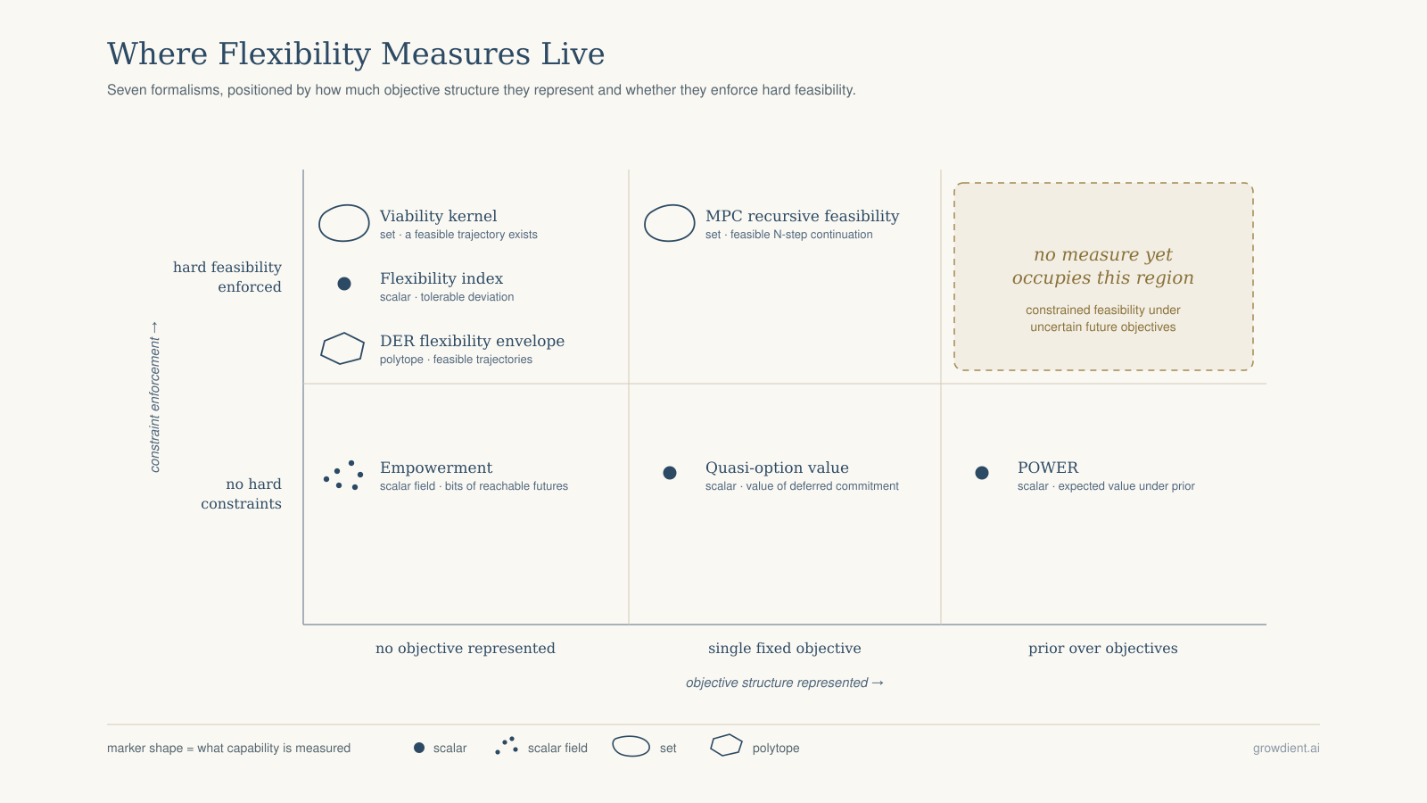
Look at which rows carry an objective prior and which enforce hard feasibility. The measures with real constraint handling (flexibility index, viability kernel, MPC, flexibility envelopes) assume the objective is fixed, known, or irrelevant. The measure with a genuine prior over objectives, POWER, has no notion of hard operational feasibility at all.

Quasi-option value might look like a counterexample on the objective axis, but its uncertainty is a payoff-relevant state variable under a known utility functional; POWER draws the entire reward function. That is the difference between a known objective with uncertain inputs and a genuine prior over objectives.

The engineering traditions built feasibility without objective uncertainty. The AI traditions built value under objective uncertainty without constraints. The intersection (what future capability do I retain, under hard constraints, when I do not yet know what I will be asked to do) is where a greenhouse controller and a DER aggregator actually live.

That intersection is comparatively underdeveloped rather than untouched, and the distinction is worth being careful about. Reward-uncertain RL, assistance games, and preference-based methods all reason under objective uncertainty; they sit near POWER, with at most soft expected-cost constraints rather than hard feasibility. Some flexibility-index work handles objective variation through multi-period formulations, without a prior. The specific combination remains open.

The honest open question is why. It may be an oversight. It may be that nobody can supply a prior over their own future objectives, in which case the gap is a statement about tractability rather than an invitation. Any program aiming at this intersection has to answer where the prior comes from (historical objective revisions, regulatory scenario sets, an operator's own contingency plans) before the formalism is worth building.

A worked example: how much battery to hold back

Consider an inspection drone deciding how much charge to reserve before a routine survey.

The conventional reserve calculation assumes the next mission is known: estimate the planned route, the energy to fly it, the return-to-dock requirement, and hold back what that mission needs. This is a full-recourse calculation wearing different clothes. It evaluates remaining capability against one revealed objective.

But an observation-driven survey exists partly to discover what should happen next. Mid-flight, the vision system may find a pest cluster, an irrigation anomaly, or a canopy region worth a second pass. The follow-up mission is not known at departure — it is produced by the flight. The reserve decision is made under a filtration, against a distribution over later objectives, and the energy is spent irreversibly before any of them is revealed.

The consequence is not a misestimated flight time. It is a reversed ranking.

Take a battery of 100 energy units, a routine survey of 80 rows, one energy unit per row, and one unit of operational value per row inspected. A reserve $r$ leaves $\min(80,\,100-r)$ rows surveyed. Two candidate policies, with every energy figure net of return-to-dock — the flight home is budgeted separately, so the reserve is fully available for follow-up work:

Policy	Reserve $r$	Rows inspected	Value, nominal objective
A: aggressive survey	20	80	80
B: conservative survey	35	65	65

Under the known-mission calculation A dominates by 15, and B's extra reserve reads as unnecessary conservatism. Now give the flight a revelation process — the follow-up mission the survey itself produces:

Observed mid-flight	Probability	Extra energy	Value if completed
No anomaly	0.50	0	0
Local rescan	0.30	25	30
Extended pest inspection	0.20	35	60

Policy A's 20-unit reserve funds neither follow-up, so it stays at 80. Policy B funds both:

$$V_B = 65 + 0.30(30) + 0.20(60) = 86 \;>\; 80 = V_A$$

The ordering flips. Nothing about the physics changed — only the question the metric was asked.

Writing the mismatch down

Let $b$ be remaining battery, $x$ the drone and greenhouse state, $\theta$ the follow-up objective drawn from a prior $\Pi$, and $\mathcal{I}$ the information pattern governing when $\theta$ is revealed. Write $\mathcal{A}_{\mathcal{I}}$ for the policies admissible under that pattern (those measurable with respect to what is actually known when each decision is taken) and $U_\theta(\pi)$ for the value of running policy $\pi$ against objective $\theta$.

The quantity the system actually needs is

$$\mathcal{F}(b, x \mid \Pi, \mathcal{I}) \;=\; \max_{\pi \,\in\, \mathcal{A}_{\mathcal{I}}} \; \mathbb{E}_{\theta \sim \Pi}\big[\, U_\theta(\pi) \;\big|\; b, x \,\big]$$

with the maximum outside the expectation, because the policy is committed before $\theta$ arrives. The nominal reserve calculation instead evaluates

$$\mathcal{F}_{\text{nominal}}(b, x) \;=\; \max_{\pi} \; U_{\bar\theta}(\pi)$$

against a single fixed $\bar\theta$. A third quantity (the one a full-recourse metric reports) puts the maximum inside:

$$\mathcal{F}_{\text{FR}}(b, x \mid \Pi) \;=\; \mathbb{E}_{\theta \sim \Pi}\Big[\, \max_{\pi} \, U_\theta(\pi) \,\Big]$$

That ordering of operators is the entire disagreement. Choosing after revelation is at least as good as choosing before:

$$\mathbb{E}_{\theta}\Big[\max_{r} V(r, \theta)\Big] \;\;\ge\;\; \max_{r}\, \mathbb{E}_{\theta}\big[V(r, \theta)\big]$$

A full-recourse metric therefore systematically overestimates achievable future value. Separately and independently, planning against one nominal objective undervalues reserve, because reserve earns nothing under $\bar\theta$. The two errors point the same direction and select a reserve that is too small.

The failure is visible in the argument of the maximum, not only its value:

$$\arg\max_{r} \, V(r, \bar\theta) \;\;\neq\;\; \arg\max_{r} \, \mathbb{E}_{\theta \sim \Pi}\big[V(r, \theta)\big]$$

This is why rank reversal is the sharp diagnostic. A metric that is biased but preserves the argmax still selects the right policy.

The vocabulary already exists

Stochastic programming formulated these problems in the 1950s and named the quantities over the decades that followed: wait-and-see against here-and-now in Madansky (1960), the value of the stochastic solution in Birge (1982). The drone example computes them exactly. The wait-and-see value assumes $\theta$ known before the reserve is fixed; the recourse problem commits first; the expected-value solution optimizes against $\bar\theta$ and is then judged by reality:

$$\underbrace{\mathbb{E}_{\theta}\Big[\max_{r} V(r,\theta)\Big]}_{\text{WS} \,=\, 96.5} \;\;\ge\;\; \underbrace{\max_{r}\, \mathbb{E}_{\theta}\big[V(r,\theta)\big]}_{\text{RP} \,=\, 86} \;\;\ge\;\; \underbrace{\mathbb{E}_{\theta}\big[V(r^{*}(\bar\theta),\, \theta)\big]}_{\text{EEV} \,=\, 80}$$

Two gaps fall out. The value of the stochastic solution, $\mathrm{VSS} = \mathrm{RP} - \mathrm{EEV} = 6$, is what the nominal-objective planner leaves on the table by refusing to represent the objective prior at all. The expected value of perfect information, $\mathrm{EVPI} = \mathrm{WS} - \mathrm{RP} = 10.5$, is what a full-recourse metric would have to hallucinate to report WS as though it were achievable.

Policy B, at $r = 35$, is exactly the recourse optimum. The nominal calculation misses it by six units of value and, more damagingly, ranks it second.

Which axes broke

Three of the four are mismatched at once, which is why the failure is severe rather than marginal.

The filtration is wrong: the calculation behaves as though the mission is known when the reserve is chosen, when the mission is generated by the flight. The objective semantics are wrong: a single fixed $\bar\theta$ replaces a prior $\Pi$ over rescan, pest inspection, and no-follow-up. The capability quantity is wrong: remaining nominal flight time is not the ability to serve observation-contingent missions, and no amount of precision in measuring the first will produce the second.

Only the uncertainty semantics survive intact — and the metric is still wrong enough to invert the decision.

What transfer failure looks like

The framework's practical payload is a prediction: a measure computed under one specification, applied under another, is miscalibrated in ways that follow from the mismatch.

Some of this is definitional. If full-recourse policies strictly contain nonanticipative ones, and the capability functional is monotone in the admissible policy set, a full-recourse measure necessarily upper-bounds the realistic one. That is monotonicity of a supremum, not a discovery. Its use is as a consistency check (an estimator that violates it is broken), not as a scientific claim.

The empirical question is magnitude, and it is wide open. How badly does a full-recourse flexibility index overstate retained capability on a system with realistic sensing delay? Does the error preserve the ranking of designs, or reorder them? A metric that is biased but rank-preserving is usable; one that reorders is worse than nothing. The drone example shows reordering is possible, but it is a two-policy construction with chosen numbers — it establishes that the failure mode exists, not that it bites at realistic parameter values on deployed systems. That remains unmeasured, because no benchmark varies these specifications systematically.

Other mismatches have no obvious sign. Widening the support of the objective prior does not monotonically change the value of preserving general-purpose capability — it depends on the capability functional. That non-monotonicity is more interesting than the ordering result, because the answer is not already known.

What is already connected

The bridges that exist are exactly the ones between communities that already shared a mathematical dialect. Viability kernels, maximal control invariant sets and Hamilton–Jacobi backward reachable sets describe the same safe sets, and reach-avoid has its own HJ formulation. Viability theory and MPC recursive feasibility have been formally related. The flexibility index has been compared directly with adjustable robust optimization — which found, usefully, that the robust formulation can be more conservative than the classical one. Control barrier functions have extended the dynamic flexibility index toward invariance.

Set-valued analysis, optimization duality and dynamic programming translate. Information theory, welfare economics and set-valued control do not, and the gaps fall exactly there. Empowerment and Aubin's mathematical viability theory have no peer-reviewed connection I could find — the artificial-life literature invokes viability around empowerment, but in the enactivist sense, without the kernel machinery: a 2025 empowerment paper on preserving controllable futures and avoiding trap states cites no viability-kernel work at all. Empowerment and quasi-option value, two formalisms for the value of keeping options open, appear in no paper I could find that cites both.

None of this is new as an observation about the field's fragmentation. Saleh, Mark & Jordan (2009) surveyed flexibility across disciplines and concluded it was "not yet an academically mature concept" relative to optimality and robustness. Seventeen years later that is substantially unmet — and the community that pushed hardest on systematization, energy systems, documented significant disparity among the mathematical formulations of flexibility models within its own borders.

What is missing is not the observation. It is a specification precise enough to say what breaks when you cross a boundary.

Where this is wrong

The classification above is a proposal, and the most useful response is a correction. Specifically:

• Which row mischaracterizes your community's measure, and in which column?
• Which flexibility measure does not fit these four axes at all?
• Have you seen a measure transferred between settings and produce a wrong answer — and did the error show up as a wrong number, or a wrong ranking?
• Where does recourse enter your definition, and is it stated or assumed?
• If you use a prior over future objectives, where does it come from?

The third question is the one worth the most. A single documented case where a flexibility metric was imported across a boundary and misled someone is worth more than any amount of agreement about the taxonomy — it is the difference between a classification and an instrument.